41 excel chart change labels

Change the format of data labels in a chart To get there, after adding your data labels, select the data label to format, and then click Chart Elements > Data Labels > More Options. To go to the appropriate area, click one of the four icons ( Fill & Line, Effects, Size & Properties ( Layout & Properties in Outlook or Word), or Label Options) shown here. Excel Custom Chart Labels - My Online Training Hub Using Excel custom chart labels is a great way to create a more insightful chart without having to show a whole other series. Just take this chart below with custom labels showing the year on year % change:

Resize the Plot Area in Excel Chart - Titles and Labels ... In the case of Tony's chart in the video, he was having trouble seeing the axis titles and labels because the plot area was too large. Therefore, the plot area needs to be smaller than the chart area to fit the axis labels, and titles outside the chart. Get Your Question Answered. This article is based on a question from Tony.

Excel chart change labels

Add or remove data labels in a chart Click the data series or chart. To label one data point, after clicking the series, click that data point. In the upper right corner, next to the chart, click Add Chart Element > Data Labels. To change the location, click the arrow, and choose an option. If you want to show your data label inside a text bubble shape, click Data Callout. Edit titles or data labels in a chart The first click selects the data labels for the whole data series, and the second click selects the individual data label. Right-click the data label, and then click Format Data Label or Format Data Labels. Click Label Options if it's not selected, and then select the Reset Label Text check box. Top of Page How to create Custom Data Labels in Excel Charts Create the chart as usual. Add default data labels. Click on each unwanted label (using slow double click) and delete it. Select each item where you want the custom label one at a time. Press F2 to move focus to the Formula editing box. Type the equal to sign. Now click on the cell which contains the appropriate label.

Excel chart change labels. Create Dynamic Chart Data Labels with Slicers - Excel Campus Typically a chart will display data labels based on the underlying source data for the chart. In Excel 2013 a new feature called "Value from Cells" was introduced. This feature allows us to specify the a range that we want to use for the labels. Since our data labels will change between a currency ($) and percentage (%) formats, we need a ... 2/ Right-click i.e. on the 1st histo. bar (A) > Add Data Labels (numbers are displayed a the top of the bars) 3/ Click one of the numbers that just displayed (the Format Data Labels pane opens on the right) > Check option "Value From Cells" > Select range C2:C7 > OK > Uncheck option "Value" demo.png (18.5 KiB) · 3 Excel charts: add title, customize chart axis, legend and ... How to change data displayed on labels To change what is displayed on the data labels in your chart, click the Chart Elements button > Data Labels > More options… This will bring up the Format Data Labels pane on the right of your worksheet. Switch to the Label Options tab, and select the option (s) you want under Label Contains: How to change chart axis labels' font color and size in Excel? Right click the axis you will change labels when they are greater or less than a given value, and select the Format Axis from right-clicking menu. 2. Do one of below processes based on your Microsoft Excel version:

How to Change Excel Chart Data Labels to Custom Values? You can change data labels and point them to different cells using this little trick. First add data labels to the chart (Layout Ribbon > Data Labels) Define the new data label values in a bunch of cells, like this: Now, click on any data label. This will select "all" data labels. Now click once again. Excel chart changing all data labels from value to series ... I am having this problem in excel stacked column chart while trying to change the labels. My graph has multiple columns and hundreds of stacked values (series) in each column. By selecting chart then from layout->data labels->more data labels options ->label options ->label contains-> (select)series name, I can only get one series name ... How to edit the label of a chart in Excel? - Stack Overflow The latter box will list the "1", "2", etc. numbers that you want to change. Hit the edit button for the right-hand box (Horizontal Category (Axis) Labels), and you will be prompted to enter an axis label range. Instead of selecting a range, though, just enter the labels that you want to see on the x-axis, separated by commas, like so: How to add data labels from different column in an Excel ... Right click the data series in the chart, and select Add Data Labels > Add Data Labels from the context menu to add data labels. 2. Click any data label to select all data labels, and then click the specified data label to select it only in the chart. 3.

Add / Move Data Labels in Charts - Excel & Google Sheets ... Adding Data Labels Click on the graph Select + Sign in the top right of the graph Check Data Labels Change Position of Data Labels Click on the arrow next to Data Labels to change the position of where the labels are in relation to the bar chart Final Graph with Data Labels Excel tutorial: How to customize axis labels Instead you'll need to open up the Select Data window. Here you'll see the horizontal axis labels listed on the right. Click the edit button to access the label range. It's not obvious, but you can type arbitrary labels separated with commas in this field. So I can just enter A through F. When I click OK, the chart is updated. Custom Data Labels with Colors and Symbols in Excel Charts ... The chart will show the upward and downward arrow instantly. 1.1.1 Problems. Problem as I said in the beginning is that though the data labels I connected will update if data changes, but if I throw additional rows to the chart, the new data labels needs to be connected too and that makes it quite cumbersome. How to display text labels in the X-axis of scatter chart ... Display text labels in X-axis of scatter chart. Actually, there is no way that can display text labels in the X-axis of scatter chart in Excel, but we can create a line chart and make it look like a scatter chart. 1. Select the data you use, and click Insert > Insert Line & Area Chart > Line with Markers to select a line chart. See screenshot: 2.

Directly Labeling Excel Charts | PolicyViz

How To Add Axis Labels In Excel [Step-By-Step Tutorial] Axis labels make Excel charts easier to understand.. Microsoft Excel, a powerful spreadsheet software, allows you to store data, make calculations on it, and create stunning graphs and charts out of your data.. And on those charts where axes are used, the only chart elements that are present, by default, include:

How do I change the order of pie chart slices?

How to rotate axis labels in chart in Excel? Go to the chart and right click its axis labels you will rotate, and select the Format Axis from the context menu. 2. In the Format Axis pane in the right, click the Size & Properties button, click the Text direction box, and specify one direction from the drop down list. See screen shot below: The Best Office Productivity Tools

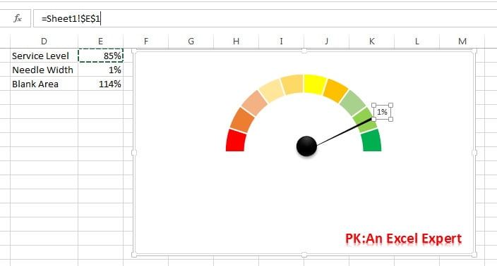
Speedometer Chart - PK: An Excel Expert

How to Customize Your Excel Pivot Chart Data Labels - dummies To add data labels, just select the command that corresponds to the location you want. To remove the labels, select the None command. If you want to specify what Excel should use for the data label, choose the More Data Labels Options command from the Data Labels menu. Excel displays the Format Data Labels pane.

Pie Chart - PK: An Excel Expert

Change axis labels in a chart in Office To change the label, you can change the text in the source data. If you don't want to change the text of the source data, you can create label text just for the chart you're working on. In addition to changing the text of labels, you can also change their appearance by adjusting formats.

How to Add Data Labels to your Excel Chart in Excel 2013 - YouTube

Excel Chart Data Labels-Modifying Orientation - Microsoft ... Replied on September 14, 2016 In reply to PaulaAB's post on September 13, 2016 Hi Paula, You can right click on the data label part then select Format Axis. Click on the Size & Properties tab then adjust the Text Direction or Custom Angle. Thanks, Mike Report abuse 6 people found this reply helpful · Was this reply helpful? Replies (7)

Waterfall Chart - Page 2 of 2 - Beat Excel!

Is there a way to change the order of Data Labels ... Microsoft Agent | Moderator Replied on April 4, 2018 Hi Keith, I got your meaning. Please try to double click the the part of the label value, and choose the one you want to show to change the order. Thanks, Rena ----------------------- * Beware of scammers posting fake support numbers here.

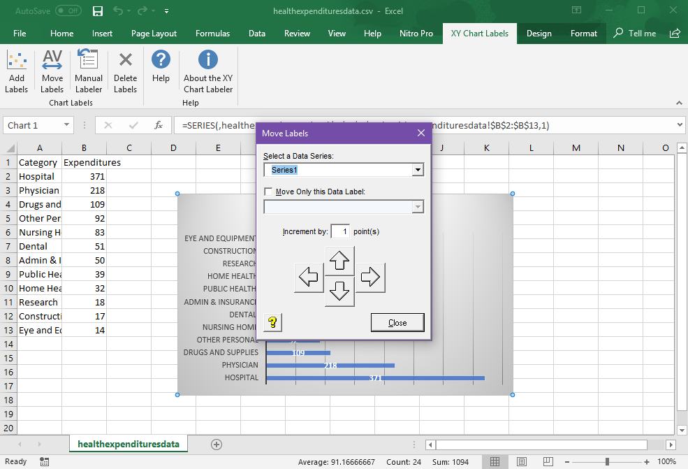
Add Labels to XY Chart Data Points in Excel with XY Chart Labeler

Individually Formatted Category Axis Labels - Peltier Tech In the column chart, you need to change the chart type of the added column series to a line chart. Format the category axis (horizontal axis) so it has no labels. Add data labels to the the dummy series.

Share :